When the Average Is Right but the Breaches Are Wrong

When the Average Is Right but the Breaches Are Wrong

An average can be correct while the conclusion drawn from it is wrong.

That matters when modelling an industrial plant required to operate below an emission limit or air-quality objective. The question is not simply whether its average emission rate appears acceptable. The question is whether the plant will remain within the applicable limits as its feed, operating conditions and emissions vary through time.

Those are different questions.

A model may estimate an average reasonably well while giving a poor estimate of the frequency, magnitude or duration of breaches. Once a regulatory threshold is involved, variability around the average is not a secondary detail.

It may determine the compliance outcome.

If that variability is understated, the problem may extend beyond the modelled concentrations. It may also mislead the assessment manager about the likely performance of the plant, the margin beneath the applicable objectives and whether the proposed conditions can adequately control the development.

Same average, different behaviour

Consider two modelled emission profiles.

Both have exactly the same average. If a report presented only that average, the two plants would appear identical.

They are not.

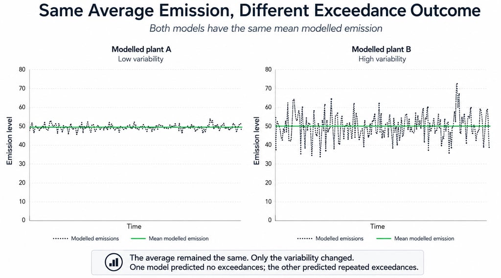
The first profile has low variability. Most results remain close to the average.

The second has much greater variability. It produces more low values, more high values and a much wider spread around exactly the same centre.

An average tells us where the centre of a distribution lies.

It does not tell us:

• how widely the results are spread;

• how frequently unusually high values occur;

• how high they may be;

• how long they may persist;

• whether they are associated with particular operating conditions; or

• whether the model represents the real behaviour of the process.

This is elementary statistics, but it is repeatedly neglected in technical assessments.

A model can estimate the centre of a distribution reasonably well while badly misrepresenting its tails.

Unfortunately, the tails are where breaches occur.

The average is not the operation

Imagine two plants that each average 50 units of emissions over a year.

The first generally operates between 45 and 55.

The second ranges between 10 and 90.

They have the same average.

They do not have the same operating performance.

If the applicable limit is 60, the first plant may remain below it throughout the year. The second may cross it repeatedly.

Nothing about the average changed.

What changed was the variability around it.

This is why compliance cannot be established merely by showing that an average result is below a limit.

An annual average says little about hourly peaks unless a defensible relationship between the two has been demonstrated.

Regulatory limits and air-quality objectives also apply over defined averaging periods. A one-hour criterion, a daily criterion and an annual criterion ask different questions.

An annual average cannot simply be presented as reassurance against short-duration events.

An average is a useful statistic.

It is not a substitute for the distribution.

Why modelled results often look tidier than reality

Real operating data are untidy.

They contain peaks, troughs, process disturbances, changing operating states, measurement noise and unusual events. They do not ordinarily sit on a neat line.

Models simplify that behaviour. That is their purpose.

But simplification commonly reduces apparent variability. High observations are pulled down towards the fitted response. Low observations are pulled up. The modelled system becomes smoother than the observed system.

That is not automatically an error.

The error occurs when decision-critical variability is removed and the resulting smoothness is then treated as evidence of stable performance.

If the purpose of a model is to estimate a long-term average, some smoothing may be acceptable.

If the purpose is to determine whether a threshold will be crossed, the tails of the distribution are central to the question.

Smoothing them away changes the question being answered.

A technically elaborate model does not cure that problem.

It may simply calculate the wrong quantity with greater precision.

Now add the red line

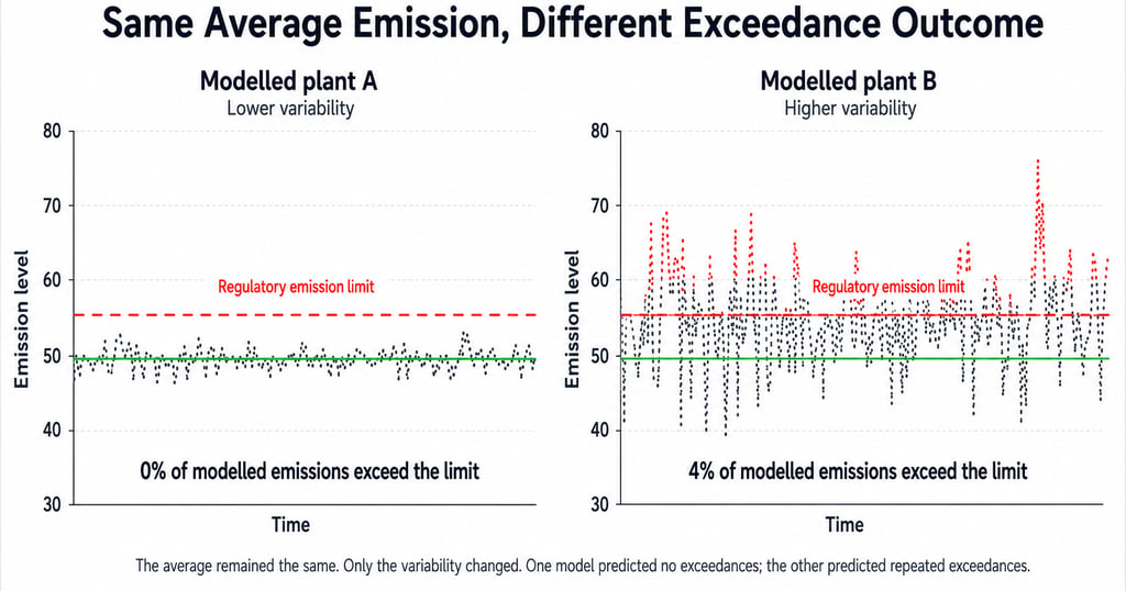
Place the same regulatory limit across both emission profiles.

In the low-variability case, every modelled result remains below the line.

In the high-variability case, the average remains unchanged, but some of the higher values cross it.

In the constructed example used in the accompanying graphic, the limit is breached during 4 per cent of the modelled periods.

That figure is illustrative. It is not a prediction of the performance of the proposed Glan Devon plant.

The point is what happened when only the variability changed.

The average remained the same.

The limit remained the same.

One model predicted complete compliance.

The other predicted repeated breaches.

A model can therefore get the average right and the regulatory conclusion wrong.

What exactly is the red line?

There can be several red lines in an air-quality assessment.

One may be a limit on emissions leaving the stack. Another may be an ambient air-quality objective applying at a residence, workplace or other receptor. Different pollutants may also have different limits and averaging periods.

Those distinctions matter, but the underlying statistical problem remains.

A dispersion model takes an assumed emission rate, combines it with weather, terrain, stack parameters and other inputs, and predicts concentrations away from the source.

If the assumed source term is unrealistically smooth, the model does not recreate the missing variability.

It calculates the consequences of the smooth source it was given.

That does not mean every concentration will necessarily be underestimated. Some may be overestimated and others underestimated. The particular effect depends on the pollutant, meteorology, timing and averaging period.

The central problem is more basic.

The model cannot correctly estimate the frequency and magnitude of peaks if the source variation responsible for those peaks is absent from the input.

CALPUFF is a dispersion model.

It is not a machine for manufacturing missing process data.

Thresholds make uncertainty consequential

Without a threshold, a small modelling error may appear relatively unimportant.

A prediction of 48 rather than 52 may not greatly alter a broad estimate of average performance.

Place a regulatory limit at 50 and the same error changes the conclusion from compliance to breach.

The threshold converts uncertainty in the model into uncertainty in the decision.

That is why the margin between the predicted result and the limit matters.

A result well below the limit may remain below it despite moderate uncertainty.

A result close to the limit is different. A modest amount of unrepresented variation may move part of the true distribution across the line.

The closer the modelled result is to the threshold, the less defensible it becomes to rely on a single smooth value without establishing the underlying distribution.

A narrow modelled margin is not necessarily evidence of safety.

It may be evidence that the conclusion is highly sensitive to assumptions that have not been tested.

A percentile is only as meaningful as the distribution beneath it

The same problem arises when the assessment presents upper percentiles of modelled concentrations.

A percentile is not simply another number.

It is a position within a distribution.

A 99th percentile means that 99 per cent of the values in the relevant distribution fall at or below that value, with 1 per cent above it.

For that statement to be useful, the distribution must represent the quantity about which the decision is being made.

That raises an obvious question:

The 99th percentile of what?

Is it the 99th percentile of measured stack emissions from sustained commercial operation?

Is it the 99th percentile of emissions across changing feedstocks, operating states, startups, shutdowns and process disturbances?

Is it the 99th percentile of predicted ground-level concentrations under variable emissions and variable weather?

Or is it the 99th percentile of concentrations produced by a dispersion model while the source emission rate remains fixed?

Those are not interchangeable.

If CALPUFF is supplied with a constant emission rate, the modelled concentrations still vary because the weather varies. A 99th percentile can therefore be calculated from the resulting concentration predictions.

Mathematically, that percentile may be perfectly correct.

But it is the 99th percentile conditional on the assumed constant source.

It represents meteorological variation within the model.

It does not represent the full variation of the operating plant.

The real concentration at a receptor depends on at least two changing systems:

• the emissions leaving the source; and

• the atmospheric conditions dispersing those emissions.

The modelled system may be represented as:

Concentration = f(constant source, changing weather)

The real system is closer to:

Concentration = f(changing source, changing process, changing weather)

If variation in the source and process has been removed, the upper percentiles calculated from the model are percentiles of a reduced system.

Calling the result a 99th percentile does not restore the missing variability.

For many familiar distributions, upper percentiles rise as variability increases even when the average remains unchanged.

Under a normal-distribution assumption, for example, the 99th percentile is approximately:

99th percentile = mean + 2.326 × standard deviation

Reduce the standard deviation and the calculated 99th percentile falls.

That is not a modelling opinion.

It is what the percentile means.

The real emissions do not need to follow a normal distribution for the underlying point to remain valid.

Waste-incinerator emissions may be skewed, heavy-tailed, multimodal or divided among distinct operating states.

Those features make reliance on a smoothed source more problematic, not less.

How this may mislead the assessment manager

The model does not necessarily determine the statutory air-quality objective. That objective may already be established through the relevant environmental framework.

The planning problem is different.

The model is used to help the assessment manager decide whether the proposed development can meet the applicable objectives and whether any remaining risk can be adequately controlled through approval conditions.

If the model understates source variability, it may give a misleading answer to those questions.

A modelled 99th-percentile concentration may appear comfortably below the applicable objective. The assessment manager may therefore conclude that:

• the proposal has an adequate compliance margin;

• the selected worst-case scenario is conservative;

• the predicted impacts are unlikely to exceed the objective;

• occasional monitoring will be sufficient;

• operational variation can be managed through conditions; or

• the proposed operating envelope has been adequately assessed.

But those conclusions depend on the modelled distribution representing the real system.

If the upper percentile was calculated from changing weather acting on a constant source, it does not establish the corresponding percentile of concentrations from a changing plant.

Its relationship to the real operating percentile is unknown.

The assessment manager may therefore be shown an apparently precise measure of upper-end performance without being told that a major source of upper-end variation has been excluded.

That is not merely uncertainty around the edges of the result.

It goes directly to the question the assessment manager is being asked to decide:

Can this development operate within the applicable limits, and can conditions reliably keep it there?

If the model has not represented the source variability, it may provide false confidence about both parts of that question.

Conditions may appear adequate because the model is incomplete

Conditions do not need to change the applicable environmental objective for this problem to arise.

They are intended to confine the approved development to an acceptable operating envelope.

If the modelled operating envelope is incomplete, the proposed conditions may appear adequate only because the model has not represented the behaviour they need to control.

For example, a smoothed model may lead the assessment manager to accept:

• a broadly defined fuel category rather than a defensible fuel specification;

• occasional stack testing rather than monitoring capable of detecting short-duration peaks;

• a single operating-temperature requirement;

• general process-management conditions;

• corrective action after a breach rather than preventive shutdown triggers; or

• a nominated emission rate that has not been shown to bound real operation.

The problem is not necessarily that any one of those conditions is inherently invalid.

The problem is that their adequacy cannot be established from a model that has omitted the source variability they are expected to manage.

A condition package may look comprehensive on paper while leaving the central operating uncertainty unresolved.

Conditions cannot correct a distribution that has never been established.

Breaches are not just marks on a chart

A breach has consequences.

For the operator, repeated breaches may mean additional testing, reporting, investigation, maintenance, interrupted production, plant modifications or shutdowns.

For regulators and council, they may mean complaints, correspondence, inspections, technical reviews, enforcement decisions and continuing pressure to act.

For neighbours, they may mean inconvenience, concern and a growing belief that the modelling and approval process cannot be trusted.

Those effects can reinforce one another.

More suspected breaches produce more complaints and investigation. Increased monitoring may then detect problems that were previously missed. That generates further concern, greater scrutiny and pressure for tighter control.

The proper response is better process control and fewer breaches.

But that assumes the operator can identify and reliably control the causes of the variation.

For an established plant with a long operating history, that proposition can be tested against evidence.

For a proposed technology processing a changing waste feed, it must be demonstrated before approval.

It should not be discovered later through complaints, investigations and enforcement.

Waste-incinerator emissions are not constant

Operating waste incinerators do not produce perfectly constant stack emissions.

Emissions change as the feed changes, combustion conditions change and the plant moves through startup, shutdown, interruption, maintenance and other operating states.

Waste composition affects moisture, calorific value, particle size and contaminant loading.

Plastics, treated timber, paints, glues, coatings, pigments, fillers and preservatives introduce different chemical and physical properties.

The plant must respond to those changes.

Feed rate, oxygen supply, temperature, residence time and pollution-control performance all operate within physical ranges.

None can reasonably be assumed to remain constant.

Published studies of waste-incineration processes report changes in emissions associated with changing feed materials and process conditions.

Regulatory practice also commonly distinguishes startup, shutdown and other-than-normal operating periods because those periods may not behave like steady normal operation.

Those studies are not evidence of the exact performance of a Xetrov furnace.

They establish the general engineering expectation:

a variable feed entering a dynamic combustion process should be expected to produce variable outputs unless evidence shows otherwise.

If Xetrov has achieved unusually stable emissions from a changing waste feed, that should be visible in operating data.

It should not need to be assumed.

Where is the Xetrov operating distribution?

This is where the issue becomes specific to Glan Devon.

I have found no publicly available, independently verifiable operating record showing how a commercial Xetrov unit performs over an extended period while processing a variable non-recyclable waste feed.

The Pollington pilot plant has been reported by East Riding Council as mothballed, with the council reporting no emissions data held.

A Xetrov installation has also been associated publicly with Daventry, but I have found no publicly verifiable operating record showing that it became a functioning commercial-scale mixed-waste facility operating over time.

More importantly, I have found no published Xetrov time series showing:

• the distribution of stack emissions;

• the spread around the average;

• the frequency and magnitude of high-emission periods;

• the relationship between feed composition and emissions;

• performance during startup and shutdown;

• performance during interrupted or unstable operation;

• the frequency of alarms or control-system interventions; or

• the frequency with which regulatory limits were approached or exceeded.

The absence of publicly available data does not prove that no data exist.

It does mean that the proposed performance cannot be checked against a demonstrated commercial operating distribution.

The “normal” and “worst-case” values used for Glan Devon therefore do not appear to be statistical summaries derived from sustained commercial Xetrov operation on the proposed feed.

There is no publicly available distribution against which either label can be tested.

What the applicant’s assessment actually uses

The applicant’s Air Quality Assessment in Appendix H, Part 2 describes the source of the Xetrov emissions inputs.

The emissions data came from a trial in which the equipment was operating at approximately 70 per cent capacity while burning polyurethane dust.

The measured results were multiplied by 1.42 to estimate emissions at full capacity.

Multiplying a measured value by 1.42 makes the number larger.

It does not create a distribution.

It does not establish variability.

It does not show what happens when the fuel changes from load to load.

It does not show how the plant responds to changing plastics, treated timber, paints, coatings, glues, preservatives, fillers, moisture or contaminants.

It does not establish what happens when several of those variables change together.

It does not establish performance during startup, shutdown, interrupted operation, equipment degradation or unstable combustion.

Scaling from 70 per cent to 100 per cent capacity assumes that emissions increase in direct proportion to throughput.

That is a testable assumption.

It is not a physical law.

The calculation answers only this:

What would the measured value become if it increased linearly with throughput?

It does not establish that the relationship is linear.

It does not establish the range of possible outcomes.

And it does not convert a test on one comparatively consistent material into evidence of performance on a changing mixed-waste fuel.

The multiplication is arithmetic.

It is not validation.

Two tidy versions of a plant that will not be tidy

The modelling pathway appears to be:

1. test one feed at approximately 70 per cent capacity;

2. scale the result to full capacity;

3. select a normal emission rate and a stated worst-case rate; and

4. hold each rate constant during a separate dispersion-model run.

That produces two source terms.

It does not produce an operating distribution for a commercial Xetrov plant processing variable non-recyclable waste.

Appendix H models a normal case and a stated worst-case case.

Within each case, the stack emission rate assigned to each pollutant appears to remain fixed through the model run.

The weather changes.

The plume changes.

The source does not.

The assessment therefore models two perfectly steady versions of the incinerator:

one always operating at the selected normal rate and one always operating at the selected worst-case rate.

A real plant will not alternate between two constant states.

It will move through a range of lower, typical, elevated, disturbed and abnormal conditions.

The modelling does not establish that range.

It does not show the spread around the selected values.

It does not show how frequently elevated conditions occur.

It does not establish whether some operating periods exceed the selected worst-case value.

Without those data, the model cannot determine how often the actual plant may approach or cross a regulatory threshold.

Critically, the value labelled “worst case” has not been shown to be a bounding value, an upper percentile from a representative operating distribution or even an observation near the upper end of the plant’s true performance range.

Without a distribution, “worst case” is not a statistical result.

It is a label.

What does the constant normal case tell us?

A constant normal case tells us what CALPUFF predicts when it is supplied with the selected normal emission rate for every modelled hour.

That is useful, but limited.

It does not establish how “normal” was defined.

It does not tell us whether the value is a mean, median, percentile, single observation or engineering judgement.

It does not tell us how often the plant may exceed it.

It does not tell us how far above it the plant may rise.

It does not establish whether high-emission periods may coincide with meteorological conditions that produce poor dispersion at particular receptors.

The weather varies in the model.

The source does not.

A real facility would have variability in both.

Unless time-varying emissions are represented, the interaction between source variation and meteorological variation has not been assessed.

What does the constant worst-case case tell us?

The phrase “worst case” sounds conservative.

It is not necessarily so.

A worst-case input is meaningful only when the basis for calling it worst case is demonstrated.

Was it the highest observation from a representative operating period?

Was it derived from a sufficiently large dataset?

Was it associated with startup, shutdown or a process disturbance?

Was it associated with a particular feed composition?

Was it selected separately for each pollutant?

What percentile does it represent?

Could higher values occur?

Without answers to those questions, the term “worst case” carries no statistical content.

Holding that rate constant may be conservative for one purpose and inadequate for another.

It may overstate a long-term average if the real plant reaches the value only occasionally.

At the same time, it may fail to represent shorter and higher peaks above that value.

It says nothing about the duration, frequency or sequence of high-emission events.

A constant worst-case run answers:

What concentrations would CALPUFF predict if the selected emission rate occurred continuously?

It does not answer:

How does the plant actually vary, and how often will that variation produce unacceptable concentrations?

Those questions should not be confused.

The timing of high emissions matters

Air impacts depend not only on how much is emitted, but also on when it is emitted.

A high-emission episode during good dispersion may produce a different ground-level concentration from the same episode during stable atmospheric conditions, low wind speeds or winds directed towards a receptor.

A constant source term tests each meteorological hour against the same emission rate.

It does not test the combined behaviour of a changing source and changing weather.

There may be no systematic relationship between process disturbances and meteorological conditions.

There may be one.

The assessment cannot establish either proposition because the source variation was not modelled.

The point is not that every omitted interaction must worsen the result.

The point is that an interaction capable of changing the threshold outcome has not been tested.

“Non-recyclable waste” is not a fuel specification

“Non-recyclable waste” is not a uniform material.

It is a broad administrative category.

It may contain different plastics, additives, pigments, fillers, treated and untreated timber, paints, glues, coatings, preservatives, moisture levels and contaminants.

The proportions may vary between trucks, stockpiles and operating days.

Milling and mixing may reduce some physical variation.

They do not make the material chemically uniform.

A mixed feed may appear visually consistent while remaining highly variable in composition.

A small amount of one material may carry a disproportionate contaminant load.

Moisture may change combustion behaviour without changing dry chemical composition.

Particle size and density may alter feed behaviour and residence time.

The plant will vary as well.

Feed rates change.

Temperatures and air flows change.

Sensors drift.

Filters load.

Equipment wears.

Control systems intervene.

None of this proves that the plant will breach a limit.

It proves that constant emissions cannot simply be assumed.

That assumption requires evidence.

Publicly available commercial Xetrov data on the proposed fuel have not been provided.

Can artificial intelligence remove the variability?

The proposal refers to artificial intelligence as part of the process-control system.

That may improve control.

It does not make the incoming waste constant, remove process delays or repeal the physical limits of the equipment.

An AI-assisted control system can respond only to variables that are measured or reliably inferred.

Its performance depends on:

• what is measured;

• measurement accuracy and frequency;

• how quickly feed changes are detected;

• the delay between a feed change and the resulting stack response;

• whether cause can be distinguished from symptom;

• the operating range of the combustion and pollution-control systems;

• the quality and relevance of the training data; and

• performance outside the conditions represented in those data.

Feedback control also acts on a process that has already changed.

Where measurement is delayed, noisy or incomplete, and where the process response is nonlinear or poorly characterised, repeated intervention can add variation rather than remove it.

That does not prove that the proposed control system will be unstable.

It means that the phrase “AI controlled” proves nothing about stability.

The required evidence is time-linked operating data showing the feed, plant state, control response and resulting stack emissions.

Without those data, “AI controlled” is a description of an intended control method.

It is not evidence of demonstrated emission performance.

Can sampling the incoming waste solve the problem?

Sampling is necessary.

It is not sufficient.

Mixed waste is difficult to sample representatively.

A small sample may miss uncommon components carrying high contaminant loads.

Material taken from one part of a truck or stockpile may not represent the remainder.

Milling reduces particle size but does not guarantee that contaminants are evenly distributed.

Sampling frequency matters.

Sample mass matters.

Sample location matters.

Preparation and analytical methods matter.

The spatial distribution of contaminants matters.

A rare but highly contaminated component may contribute little to the average stockpile composition while producing a significant short-term effect when it enters the furnace.

But there is a more fundamental problem.

Even exhaustive knowledge of the feed would not, by itself, determine the stack emissions.

The outcome depends on the feed and the state of the process when that feed is burned.

Relevant variables include feed rate, moisture, particle size, temperature, oxygen availability, residence time, mixing, combustion stability, equipment condition and pollution-control performance.

Those relationships are unlikely to be purely linear.

Why averaging the feed may not average the emissions

For a linear process, calculating the output from the average input gives the same result as calculating each output and then averaging them.

For a nonlinear process, that convenient equivalence does not generally hold:

E[f(X)] ≠ f(E[X])

Where the response is convex over the relevant range, Jensen’s inequality tells us:

E[f(X)] ≥ f(E[X])

In plain language, the average emissions produced by a varying feed may be greater than the emissions calculated from the average feed.

Suppose contaminant concentration moves between low and high values and the emission response curves upwards.

The high-concentration periods then contribute disproportionately to total emissions.

The average contaminant concentration may be calculated perfectly.

The emission calculated from that average may still be too low.

Jensen’s inequality does not prove that every form of variability increases emissions.

The direction and magnitude depend on the actual response function.

A combustion process may contain convex, concave, approximately linear and threshold-like regions.

That qualification does not weaken the argument.

It is the argument.

Without evidence describing the response function, averaging the input is not a defensible substitute for modelling the variable process.

The same problem applies to interactions between variables.

A given chlorine concentration may produce one result during stable high-temperature combustion and another when moisture rises, temperature falls or residence time changes.

Two loads with the same laboratory composition may therefore produce different emissions because they encounter different plant conditions.

This is not merely variable feed entering a fixed process.

It is variable feed entering a variable, nonlinear and state-dependent process.

Knowing the feed is necessary.

It is not sufficient.

A defensible assessment needs evidence of the plant’s transfer behaviour: how changes in the feed and process state propagate through the furnace and pollution-control system and appear at the stack.

That requires sufficiently long, time-linked operating data connecting:

• feed composition and physical properties;

• feed rate and process conditions;

• control-system responses;

• combustion and pollution-control performance; and

• continuously or frequently measured stack emissions.

Without that linkage, feed sampling establishes what entered the process.

It does not establish what left it.

Monitoring after approval is not evidence before approval

It may be argued that variability can be managed through licence conditions, stack testing and operational monitoring.

Monitoring is necessary.

It does not repair an inadequate pre-approval model.

Monitoring after operation begins tells us what the plant has already done.

It may detect a problem.

It does not necessarily prevent one.

If the approval relies on a model that has not represented the likely operating variability, the community and regulator may be left to discover the missing distribution after the facility has been built.

By then, capital has been invested.

People may be employed.

Contracts may depend on continued operation.

Waste may already be arriving.

Modification, enforcement or shutdown becomes more difficult.

That is precisely why the evidence should be required before approval.

Approving first and discovering the operating distribution later is not a conservative assessment approach.

It is commissioning the plant through trial and error, with the regulatory system and surrounding community carrying part of the risk.

Conditions cannot manufacture missing knowledge

Approval conditions are useful only when they are tied to measurable and enforceable limits.

A condition requiring the plant to operate generally in accordance with the application does not resolve uncertainty about what normal operation means.

Occasional stack testing may miss short-duration peaks.

A broad feed specification may be ineffective if it is poorly sampled or not linked to pollutant behaviour.

A temperature condition may not control contaminants arising from changing feed chemistry.

A condition requiring corrective action after a breach still allows the breach to occur.

Conditions would need to define the actual operating envelope, including:

• permitted and prohibited feed materials;

• feed preparation requirements;

• sampling methods and frequency;

• operating limits;

• startup and shutdown procedures;

• monitoring requirements;

• alarm and shutdown triggers;

• reporting obligations; and

• consequences for leaving the demonstrated envelope.

Even then, the assessment manager needs evidence showing which variables matter, how the plant actually varies and whether the conditions correspond to the operating behaviour represented in the model.

If the modelled source is smoother than the real source, the proposed conditions may appear sufficient only because the assessment has understated what must be controlled.

Conditions cannot compensate for missing process knowledge by instructing the operator to manage whatever the assessment failed to characterise.

What the Glan Devon model actually tells us

The Glan Devon assessment shows what CALPUFF predicts when supplied with two selected constant stack-emission rates.

It combines those source terms with its representation of weather, terrain, stack characteristics and receptors.

The calculations may be internally correct for the inputs supplied.

That is not the same as demonstrating that the inputs represent the proposed plant.

CALPUFF cannot establish the operating distribution of a Xetrov furnace.

It cannot create source variability that was not included.

It cannot determine the effect of a changing mixed-waste feed when that relationship has not been measured or justified.

It cannot calculate the frequency of high-emission periods from two constant cases.

It cannot establish the upper percentiles of real operation if the source distribution is absent.

And it cannot establish the frequency of regulatory breaches without a defensible time-varying source term.

This is not primarily a criticism of CALPUFF.

It is a criticism of what CALPUFF was asked to model and of the conclusions then drawn from the result.

What the assessment does not establish

Based on the publicly available material considered here, the assessment does not establish:

• the expected distribution of Xetrov stack emissions;

• the variability around the selected normal rate;

• the frequency and magnitude of elevated emissions;

• a statistical basis for describing the selected higher rate as worst case;

• the effect of realistic changes in the proposed waste feed;

• performance during startup, shutdown and disturbed operation;

• whether short-duration peaks above the modelled rates are possible;

• how effectively the proposed control system limits those peaks;

• whether modelled upper percentiles represent the upper percentiles of real operation;

• whether the margin beneath the applicable air-quality objectives is reliable; or

• how frequently the plant may approach or cross applicable limits.

These are not peripheral details.

Once compliance depends on a threshold, they are the substance of the assessment.

The questions that still require answers

What is the expected distribution of stack emissions from a commercial Xetrov plant processing the proposed non-recyclable waste?

What evidence supports that distribution?

How many operating hours, cycles, feed changes, startups, shutdowns and disturbances are represented?

How do emissions respond to changes in feed composition, moisture and physical properties?

How were the normal and worst-case values defined?

Are they means, medians, percentiles, maxima, individual tests or engineering judgements?

What is the evidence that emissions scale linearly from 70 per cent to full capacity?

What occurs during startup, shutdown, interruption and process disturbance?

Were realistic time-varying emissions used in the dispersion model?

What population and distribution underlie any reported percentile?

Does a reported 99th percentile represent the full operating system, or only modelled weather acting on a constant source?

What evidence shows that the control system can detect and manage rapid feed changes?

What evidence shows that Xetrov controls the variability observed in other waste-incineration processes?

Would the proposed approval conditions legally and practically confine the eventual plant to the operating envelope represented by the model?

And what evidence allows the assessment manager to conclude that those conditions will control the variability that the model itself has not represented?

Until those questions are answered, the assessment provides two tidy emission rates derived from limited test information.

The weather varies.

The terrain varies.

The plume varies.

Within each modelled case, the incinerator does not.

That is not a realistic representation of an operating waste-incineration plant.

The average may be right.

The modelled percentile may be mathematically correct.

The assessment manager may still be shown the wrong picture of compliance.

And the number of breaches may still be wrong.

© 2026. All rights reserved.